1. Introduction¶

The Unified Forecast Systems (UFS) Utilities repository contains pre-processing programs for the UFS weather model. These programs set up the model grid and create coldstart initial conditions. The repository is hosted on Github. Information on checking out the code and making changes to it is available on the repository wiki page.

2. Grid Generation¶

The following programs are used to create a grid.

make_hgrid

regional_esg_grid

make_solo_mosaic

orog

orog_gsl (optional)

inland (optional)

lakefrac (optional)

global_equiv_resol

shave

filter_topo

sfc_climo_gen

The grid generation process is run by these scripts (located under ./ush)

fv3gfs_grid_driver.sh (driver script)

fv3gfs_make_grid.sh (creates the geo-referencing for the grid)

fv3gfs_make_orog.sh (creates the land-sea mask, terrain and EMC gravity wave drag fields)

fv3gfs_make_orog_gsl.sh (creates GSL gravity wave drag fields)

fv3gfs_make_lake.sh (adds lakes and lake depth. optional)

fv3gfs_filter_topo.sh (filters the orography)

sfc_climo_gen.sh (creates climatological surface fields, such as soil type)

3. Description of each program¶

3.1. chgres_cube¶

3.1.1. Introduction¶

The chgres_cube program creates initial condition files to coldstart the forecast model. The initial conditions are created from either Finite-Volume Sphere (FV3) Global Forecast System (GFS), North American Mesoscale Forecast System (NAM), Rapid Refresh (RAP), or High Resolution Rapid Refresh (HRRR) gridded binary version 2 (GRIB2) data.

3.1.2. Code structure¶

Note on variable names: “input” refers to the data input to the program (i.e., GRIB2, NEMSIO, NetCDF). “Target” refers to the target or FV3 model grid. See routine doc blocks for more details.

The program assumes Noah/Noah-MP LSM coefficients for certain soil thresholds. In the future, an option will be added to use RUC LSM thresholds.

chgres.F90 - This is the main driver routine.

program_setup.F90 - Sets up the program execution.

Reads program namelist

Computes required soil parameters

Reads the variable mapping (VARMAP) table.

model_grid.F90 - Sets up the ESMF grid objects for the input data grid and target FV3 grid.

static_data.F90 - Reads static surface climatological data for the target FV3 grid (such as soil type and vegetation type). Time interpolates time-varying fields, such as monthly plant greenness, to the model run time. Set path to these files via the fix_dir_target_grid namelist variable.

write_data.F90 - Writes the tiled and header files expected by the forecast model.

atm_input_data.F90 - Contains routines to read input atmospheric data from GRIB2, NEMSIO and NetCDF files.

nst_input_data.F90 - Contains routines to read input NSST data from NEMSIO and NetCDF files.

sfc_input_data.F90 - Contains routines to read input surface data from GRIB2, NEMSIO and NetCDF files.

utils.F90 - Contains utility routines, such as error handling.

grib2_util.F90 - Routines to (1) convert from RH to specific humidity; (2) convert from omega to dzdt. Required for GRIB2 input data.

atmosphere.F90 - Process atmospheric fields. Horizontally interpolate from input to target FV3 grid using ESMF regridding. Adjust surface pressure according to terrain differences between input and target grid. Vertically interpolate to target FV3 grid vertical levels. Description of main routines:

read_vcoord_info - Reads model vertical coordinate definition file (as specified by namelist variable vcoord_file_target_grid).

newps - Computes adjusted surface pressure given a new terrain height.

newpr1 - Computes 3-D pressure given an adjusted surface pressure.

vintg - vertically interpolate atmospheric fields to target FV3 grid.

vintg_wam - vertically interpolate atmospheric fields to the thermosphere. Supports the Whole Atmosphere Model.

atmosphere_target_data.F90 - Holds the target grid atmospheric ESMF fields.

surface.F90 - process land, sea/lake ice, open water/Near Sea Surface Temperature (NSST) fields. NSST fields are not available when using GRIB2 input data. Description of main routines:

interp - horizontally interpolate fields from input to target FV3 grid.

calc_liq_soil_moisture - compute liquid portion of total soil moisture.

adjust_soilt_for_terrain - adjust soil temperature for large differences between input and target FV3 grids.

rescale_soil_moisture - adjust total soil moisture for differences between soil type on input and target FV3 grids. Required to preserve latent/sensible heat fluxes.

roughness - set roughness length at land and sea/lake ice. At land, a vegetation type-based lookup table is used.

qc_check - some consistency checks.

surface_target_data.F90 - Holds the target grid surface ESMF fields.

search_util.F90 - searches for the nearest valid land/non-land data where the input and target fv3 land-mask differ. Example: when the target FV3 grid depicts an island that is not resolved by the input data. If nearby valid data is not found, a default value is used.

thompson_mp_climo_data.F90 - Processes climatological Thompson micro-physics fields.

wam_climo_data.f90 - Process vertical profile climatological data for the Whole Atmosphere Model.

3.1.3. Configuring and using chgres_cube for global applications¶

3.1.3.1. Program inputs and outputs for global applications¶

Inputs

Users may create their own global grids, or use the pre-defined files located in the ./CRES directories. (where CRES is the atmospheric resolution and mxRES is the ocean resolution).

FV3 mosaic file - (NetCDF format)

CRES_mosaic.nc

FV3 grid files - (NetCDF format)

CRES_grid.tile1.nc

CRES_grid.tile2.nc

CRES_grid.tile3.nc

CRES_grid.tile4.nc

CRES_grid.tile5.nc

CRES_grid.tile6.nc

FV3 orography files - (NetCDF format)

CRES.mxRES_oro_data.tile1.nc

CRES.mxRES_oro_data.tile2.nc

CRES.mxRES_oro_data.tile3.nc

CRES.mxRES_oro_data.tile4.nc

CRES.mxRES_oro_data.tile5.nc

CRES.mxRES_oro_data.tile6.nc

FV3 surface climatological files - Located under the ./CRES/sfc subdirectories. One file for each tile. NetCDF format.

CRES.mxRES.facsf.tileX.nc (fractional coverage for strong/weak zenith angle dependent albedo)

CRES.mxRES.maximum_snow_albedo.tileX.nc (maximum snow albedo)

CRES.mxRES.slope_type.tileX.nc (slope type)

CRES.mxRES.snowfree_albedo.tileX.nc (snow-free albedo)

CRES.mxRES.soil_type.tileX.nc (soil type)

CRES.mxRES.subtrate_temperature.tileX.nc (soil substrate temperature)

CRES.mxRES.vegetation_greenness.tileX.nc (vegetation greenness)

CRES.mxRES.vegetation_type.tileX.nc (vegetation type)

FV3 vertical coordinate file. Text file. Located here.

global_hyblev.l$LEVS.txt

Input data files. GRIB2, NEMSIO or NetCDF. See the next section for how to find this data.

Outputs

Atmospheric coldstart files. NetCDF.

out.atm.tile1.nc

out.atm.tile2.nc

out.atm.tile3.nc

out.atm.tile4.nc

out.atm.tile5.nc

out.atm.tile6.nc

Surface/Near Sea Surface Temperature (NSST) coldstart files. NetCDF

out.sfc.tile1.nc

out.sfc.tile1.nc

out.sfc.tile1.nc

out.sfc.tile1.nc

out.sfc.tile1.nc

out.sfc.tile1.nc

3.1.3.2. Where to find GFS GRIB2 and NetCDF data for global applications¶

GRIB2

0.25-degree data (last 10 days only) - Use the gfs.tHHz.pgrb2.0p25.f000 files in subdirectory ./gfs.YYYYMMDD/HH/atmos on NOMADS.

0.5-degree data - Use the gfs_4_YYYYMMDD_HHHH_000.grb2 file, under GFS Forecasts 004 (0.5-deg) here: NCEI - Global Forecast System. Note: Tests were not done with the AVN, MRF or analysis data.

1.0-degree data - Use the gfs_3_YYYYMMDD_HHHH_000.grb2 file, under GFS Forecasts 003 (1.0-deg) here: NCEI - Global Forecast System. Note: Tests were not done with the AVN, MRF or analysis data.

NetCDF

T1534 gaussian (last 10 days only) - Use the gfs.tHHz.atmanl.nc (atmospheric fields) and gfs.tHHz.sfcanl.nc (surface fields) files in subdirectory ./gfs.YYYYMMDD/HH/atmos on NOMADS.

3.1.3.3. Initializing global domains with GRIB2 data - some caveats¶

Keep these things in mind when using GFS GRIB2 data for model initialization.

GRIB2 data does not contain the fields needed for the Near Sea Surface Temperature (NSST) scheme. See the next section for options on running the forecast model in this situation.

Data is coarse (in vertical and horizontal) compared to the NCEP operational GFS . May not provide a good initialization (especially for the surface). Recommendations:

C96 - use 0.25, 0.5 or 1.0-degree GRIB2 data

C192 - use 0.25 or 0.5-degree GRIB2 data

C384 - use 0.25-degree GRIB2 data

C768 - try the 0.25-degree GRIB2 data. But it may not work well.

Sea/lake ice thickness and column temperatures are not available. So, nominal values of 1.5 m and 265 K are used.

Soil moisture in the GRIB2 files is created using bilinear interpolation and, therefore, may be a mixture of values from different soil types. Could result in poor latent/sensible heat fluxes.

Ozone is not available at all isobaric levels. Missing levels are set to a nominal value defined in the variable mapping (VARMAP) file (1E-07).

Only tested with GRIB2 data from GFS v14 and v15 (from 12z July 19, 2017 to current). May not work with older GFS data. Will not work with GRIB2 data from other models.
Note that when concatenating grib2 files for use in initialization of global simulations, it is possible to inadvertently introduce duplicate variables and levels into the subsequent grib2 files. Chgres_cube will automatically fail with a warning message indicating that the grib2 file used contains these duplicate entries. Prior to continuing it will be necessary to strip out duplicate entries. Users can remove these entries through use of wgrib2, such as in the following command:
wgrib2 IN.grb -submsg 1 | unique.pl | wgrib2 -i IN.grb -GRIB OUT.grb, where IN.grb is the original concatenated grib2 file, and OUT.grb is the resulting grib2 file, with duplicates removed. The “unique.pl” Perl script is as follows, taken from the Tricks for wgrib2 website:
----------------------- unique.pl ------------------------
#!/usr/bin/perl -w
# print only lines where fields 3..N are different
#
while (<STDIN>) {
   chomp;
   $line = $_;
   $_ =~ s/^[0-9.]*:[0-9]*://;
   if (! defined $inv{$_}) {
     $inv{$_} = 1;
     print "$line\n";
   }
}
--------------------- end unique.pl ----------------------

3.1.3.4. Near Sea Surface Temperature (NSST) data and GRIB2 initialization¶

The issue with not having NSST data is important. In GFS we use the foundation temperature (Tref) and add a diurnal warming/cooling layer using NSST. This is the surface temperature that is passed to the atmospheric boundary layer. This is a critical feature, especially when we are doing Data Assimilation.

When using NEMSIO or NetCDF data to initialize the model, both the foundation and surface temperature are available and the atmospheric model should be run using the NSST option as this will properly account for in the forward run of the model.

In GRIB2 files only the Tsfc is stored and that is set as foundation temperature as well. So the diurnal heating / cooling is baked into the initial condition for the extent of the run. This can be critical if the model is being initialized when the ocean is warm and initialization is occuring at the peak of the diurnal warming. That warm ocean will be baked in for the extent of the run and may spawn off a number of fake hurricanes. The user has two options – either to use a spin up cycle to spin up NSST (set nstf_name = [2,1,0,0,0] in input.nml of the model namelist file. This will create a diurnal cycle after 24 hours of spin up), or to run the model without any NSST option ( set nstf_name = [0,0,0,0,0] in input.nml of the model namelist file. The user will also have to choose one of the no NSST physics suite options in input.nml).

Note, that neither of these two options will get rid of the underlying baked in heating/cooling in the surface temperature fields. For most cases this may not be an issue, but where it is then the user will either have to initialize the model with NEMSIO or NetCDF data, or replace the surface temperature in the GRIB2 fields with independently obtained foundation temperature.

3.1.3.5. Global chgres_cube namelist options¶

Namelist variables with “input” in their name refer to data input to chgres_cube. Namelist variables with “target” in their name refer to the FV3 horizontal and vertical grid (i.e., the target grid chgres_cube is mapping to).

Namelist settings for using GRIB2 data as input in global chgres_cube applications

fix_dir_target_grid - Path to the tiled FV3 surface climatological files (such as albedo).

mosaic_file_target_grid - Path and name of the FV3 mosaic file.

orog_dir_target_grid - directory containing the tiled FV3 orography and grid files (NetCDF).

orog_files_target_grid - names of the six tiled FV3 orography files.

vcoord_file_target_grid - path and name of the model vertical coordinate definition file (“global_hyblev.l$LEVS.txt).

data_dir_input_grid - directory containing the GRIB2 initial conditions data

grib2_file_input_grid - name of the GRIB2 input data file

varmap_file - path and name of the variable mapping (VARMAP) table. See below for details on this table.

input_type - input data type. Set to ‘grib2’

cycle_mon/day/hour - month/day/hour of your model initialization

convert_atm - set to ‘true’ to process the atmospheric fields

convert_sfc - set to ‘true’ to process the surface fields

Namelist settings for using NEMSIO data as input in global chgres_cube applications

fix_dir_target_grid - Path to the tiled FV3 surface climatological files (such as albedo).

mosaic_file_target_grid - Path and name of the FV3 mosaic file.

orog_dir_target_grid - directory containing the tiled FV3 orography and grid files (NetCDF).

orog_files_target_grid - names of the six tiled FV3 orography files.

vcoord_file_target_grid - path and name of the model vertical coordinate definition file (“global_hyblev.l$LEVS.txt).

data_dir_input_grid - directory containing the NEMSIO input data

atm_files_input_grid - name of the NEMSIO input atmospheric data file

sfc_files_input_grid - name of the NEMSIO input surface/Near Sea Surface Temperature (NSST) data file

input_type - input data type. Set to ‘gaussian_nemsio’.

cycle_mon/day/hour - month/day/hour of your model run

convert_atm - set to ‘true’ to process the atmospheric fields

convert_sfc - set to ‘true’ to process the surface fields

convert_nst - set to ‘true’ to process NSST fields

tracers_input - names of tracer records in input file. For GFDL microphysics, set to “spfh”,”clwmr”,”o3mr”,”icmr”,”rwmr”,”snmr”,”grle”.

tracers - names of tracer records in output file expected by model. For GFDL microphysics, set to “sphum”,”liq_wat”,”o3mr”,”ice_wat”,”rainwat”,”snowwat”,”graupel”.

Namelist settings for using NetCDF data as input in global chgres_cube applications

fix_dir_target_grid - Path to the tiled FV3 surface climatological files (such as albedo).

mosaic_file_target_grid - Path and name of the FV3 mosaic file.

orog_dir_target_grid - directory containing the tiled FV3 orography and grid files (NetCDF).

orog_files_target_grid - names of the six tiled FV3 orography files.

vcoord_file_target_grid - path and name of the model vertical coordinate definition file (“global_hyblev.l$LEVS.txt).

data_dir_input_grid - directory containing the NetCDF input data

atm_files_input_grid - name of the NetCDF input atmospheric data file

sfc_files_input_grid - name of the NetCDF input surface/Near Sea Surface Temperature (NSST) data file

input_type - input data type. Set to ‘gaussian_netcdf’.

cycle_mon/day/hour - month/day/hour of your model run

convert_atm - set to ‘true’ to process the atmospheric fields

convert_sfc - set to ‘true’ to process the surface fields

convert_nst - set to ‘true’ to process NSST fields

tracers_input - names of tracer records in input file. For GFDL microphysics, set to “spfh”,”clwmr”,”o3mr”,”icmr”,”rwmr”,”snmr”,”grle”.

tracers - names of tracer records in output file expected by model. For GFDL microphysics, set to “sphum”,”liq_wat”,”o3mr”,”ice_wat”,”rainwat”,”snowwat”,”graupel”.

3.1.4. Configuring and using chgres_cube for regional applications¶

3.1.4.1. Regional program inputs and outputs¶

Inputs

The following four sets of files/directories should all be located in the same directory (orog_dir_target_grid in the namelist):

FV3 mosaic file - (NetCDF format)

CRES_mosaic.halo4.nc

FV3 grid files - (NetCDF format)

CRES_grid.tile7.halo4.nc

FV3 orography files - (NetCDF format)

CRES_oro_data.tile7.halo4.nc

FV3 surface climatological files - NetCDF format. Linked without the “halo4” (e.g., CRES.facsf.tile7.halo4.nc linked as CRES.facsf.tile7.nc)

CRES.facsf.tile7.halo4.nc (fractional coverage for strong/weak zenith angle dependent albedo)

CRES.maximum_snow_albedo.tile7.halo4.nc (maximum snow albedo)

CRES.slope_type.tile7.halo4.nc (slope type)

CRES.snowfree_albedo.tile7.halo4.nc (snow-free albedo)

CRES.soil_type.tile7.halo4.nc (soil type)

CRES.subtrate_temperature.tile7.halo4.nc (soil substrate temperature)

CRES.vegetation_greenness.tile7.halo4.nc (vegetation greenness)

CRES.vegetation_type.tile7.halo4.nc (vegetation type)

FV3 vertical coordinate file. Text file. Located here.

global_hyblev.l$LEVS.txt

Input data files. GRIB2 only. See the next section for how to find this data.

Outputs

Atmospheric coldstart file. NetCDF. * out.atm.tile7.nc

Surface coldstart file. NetCDF. * out.sfc.tile7.nc

3.1.4.2. Where to find FV3GFS, NAM, HRRR, and RAP GRIB2 data for regional applications¶

FV3GFS

0.25-degree data (last 10 days only) - Use the gfs.tHHz.pgrb2.0p25.f000 files in subdirectory ./gfs.YYYYMMDD/HH/atmos on NOMADS.

0.5-degree data - Use the gfs_4_YYYYMMDD_HHHH_000.grb2 file, under GFS Forecasts 004 (0.5-deg) here: NCEI - Global Forecast System. Note: Tests were not done with the AVN, MRF or analysis data.

1.0-degree data - Use the gfs_3_YYYYMMDD_HHHH_000.grb2 file, under GFS Forecasts 003 (1.0-deg) here: NCEI - Global Forecast System. Note: Tests were not done with the AVN, MRF or analysis data.

NAM

12-km data from last few days (NOMADS) - Use the nam.tHHz.conusnest.hiresfHH.tmHH.grib2 files in subdirectory nam.YYYYMMDD on NOMADS.

12-km data starting 2020 - Use the nam_218_YYYYMMDD_HHHH_000.grb2 file, under NAM Forecasts NAM-NMM 218 (12km) Domain here: NCEI - North American Mesoscale Forecast System.

12-km archived data prior to 2020 can be requested through the Archive Information Request System here.

HRRR

3-km operational data from previous few days (NOMADS) - Use the hrrr.tHHz.wrfnatfHH.grib2 files in the subdirectory ./hrrr.YYYYMMDD/conus here.

3-km operational data from 2015 to present (AWS S3): Go here and click “Browse Bucket.” Type “YYYYMMDD” in to the Search bar. Use the hrrr.t00z.wrfnatf00.grib2 files in the directory hrrr.YYYYMMDD/conus/.

3-km operational data from 2015 to present (Google Cloud): Go here and click “View Dataset.” Type “hrrr.YYYYMMDD” into the “Filter” box. Use the hrrr.tHHz.wrfnatfFF.grib2 files in the hrrr.YYYYMMDD/conus directory.

3-km operational data from 2016 to present (University of Utah): Click here.

RAP

13-km operational data for the previous few days (NOMADS): Use the rap.tHHz.wrfnatfHH.grib2 files in the subdirectory ./rap.YYYYMMDD here.

13-km isobaric level data from previous 6 months : Use the rap_130_YYYYMMDD_HHHH_0FF.grb2 files from RAP Forecasts - RAP 130 (13km) - Domain at NCEI here.

13-km archived isobaric data older than 6 months can be requested through the Archive Information Request System here.

3.1.4.3. Initializing regional domains with GRIB2 data - some caveats¶

Keep these things in mind when using FV3GFS GRIB2 data for model initialization:

GRIB2 data does not contain the fields needed for the Near Sea Surface Temperature (NSST) scheme.

External model recommendations for pre-defined CONUS grids:

3-km domain, HRRR or RAP data is recommended

13-km domain: RAP or GFS data is recommended

25-km domain: GFS data is recommended

Sea/lake ice thickness and column temperatures are not available. So, nominal values of 1.5 m and 265 K are used.

For FV3GFS GRIB2 data, soil moisture is created using bilinear interpolation and, therefore, may be a mixture of values from different soil types. Could result in poor latent/sensible heat fluxes.

Ozone is not available at all isobaric levels. Missing levels are set to a nominal value defined in the variable mapping (VARMAP) file (1E-07).

Only tested with GRIB2 data from FV3GFS, RAP, NAM, and HRRR data. May not work with GRIB2 data from other models. Use these at your own risk.
Note that when concatenating grib2 files for use in initialization of regional simulations, it is possible to inadvertently introduce duplicate variables and levels into the subsequent grib2 files. Chgres_cube will automatically fail with a warning message indicating that the grib2 file used contains these duplicate entries. Prior to continuing it will be necessary to strip out duplicate entries. Users can remove these entries through use of wgrib2, such as in the following command:
wgrib2 IN.grb -submsg 1 | unique.pl | wgrib2 -i IN.grb -GRIB OUT.grb, where IN.grb is the original concatenated grib2 file, and OUT.grb is the resulting grib2 file, with duplicates removed. The “unique.pl” Perl script is as follows, taken from the Tricks for wgrib2 website:
----------------------- unique.pl ------------------------
#!/usr/bin/perl -w
# print only lines where fields 3..N are different
#
while (<STDIN>) {
   chomp;
   $line = $_;
   $_ =~ s/^[0-9.]*:[0-9]*://;
   if (! defined $inv{$_}) {
     $inv{$_} = 1;
     print "$line\n";
   }
}
--------------------- end unique.pl ----------------------

3.1.4.4. Regional chgres_cube namelist options¶

Namelist variables with “input” in their name refer to data input to chgres_cube. Namelist variables with “target” in their name refer to the FV3-LAM horizontal and vertical grid (i.e., the target grid chgres_cube is mapping to).

Required Entries

fix_dir_target_grid - Path to the FV3-LAM surface climatological files (such as albedo).

mosaic_file_target_grid - Path and name of the FV3-LAM mosaic file.

orog_dir_target_grid - Directory containing the FV3-LAM orography and grid files (NetCDF).

orog_files_target_grid - Names of the FV3-LAM orography file.

vcoord_file_target_grid - Path and name of the model vertical coordinate definition file (“global_hyblev.l$LEVS.txt).

data_dir_input_grid - Directory containing the GRIB2 initial conditions data

grib2_file_input_grid - Name of the GRIB2 input data file

varmap_file - Path and name of the variable mapping (VARMAP) table. See below for details on this table.

input_type - Input data type. Set to ‘grib2’

cycle_mon/day/hour - Month/day/hour of your model initialization

convert_atm - Set to ‘true’ to process atmospheric fields

convert_sfc - Set to ‘true’ to process surface fields

regional

Set to 0 to create initial condition atmospheric file

Set to 1 to create initial condition atmospheric file and zero hour boundary condition file

Set to 2 to create a boundary condition file. Use this option for all but the initialization time.

halo_blend - Integer number of row/columns to apply halo blending into the domain, where model and lateral boundary tendencies are applied.

halo_bndy - Integer number of rows/columns that exist within the halo, where pure lateral boundary conditions are applied.

external_model - Name of source model for input data. Valid options: ‘GFS’, ‘NAM’, ‘RAP’, ‘HRRR’, ‘RRFS’. (Default: ‘GFS’)

Optional Entries

geogrid_file_input_grid - Full path to the RAP or HRRR geogrid file corresponding to the external model input data. Only used with external_model = ‘HRRR’ or ‘RAP’.

nsoill_out - Number of soil levels to produce in the sfc_data.nc file (Default: 4).

sotyp_from_climo - Use soil type from climatology. Valid options: .true. or .false. (Default: .true.)

vgtyp_from_climo - Use vegetation type from climatology. Valid Options: .true. or .false. (Default: .true.)

vgfrc_from_climo - Use vegetation fraction from climatology. Valid options: .true. or .false. (Default: .true.)

lai_from_climo - Use leaf area index from climatology. Valid options: .true. or .false. (Default: .true.)

minmax_vgfrc_from_climo - Use min/max vegetation fraction from climatology. Valid options: .true. or .false. (Default: .true.)

tg3_from_soil - Use tg3 from input soil. Valid options: .true. or .false. . Default: .false.

thomp_mp_climo_file - Location of Thompson aerosol climatology file. Provide only if you wish to use these aerosol variables.

wam_cold_start - Cold start for the Whole Atmosphere Model. Valid Options: .true. or .false. (Default: .false.)

use_rh - Use relative humidity instead of specific humidity when reading in external model grib2 files (Default: .false.)

calrh - Type of relative humidity to specific humidity calculation to use (Default: 0; use existing calculation, or 1; use calculation consistent with GFSv15/v16)

3.1.5. Variable Mapping (VARMAP) table¶

The VARMAP table, set in the chgres_cube namelist (variable varmap_file), controls how chgres_cube handles variables that might be missing from the GRIB2 files. Since there are so many different versions of GRIB2 files, it’s often uncertain what fields are available even if you know what source model the data is coming from. Each file contains the following: (Note, only the GFS physics suite is currently supported.)

Column 1: Name the code searches for in the table. Do not change. Some definitions:

dzdt - vertical velocity

sphum - specific humidity

liq_wat - liquid water mixing ratio

o3mr - ozone mixing ratio

ice_wat - ice water mixing ratio

rainwat - rain water mixing ratio

snowwat - snow water mixing ratio

graupel - graupel mixing ratio

vtype - vegetation type

sotype - soil type

vfrac - plant greenness fraction

fricv - friction velocity

sfcr - roughness length

tprcp - precipitation rate

ffmm - surface exchange coefficient for momentum

ffhh - surface exchange coefficient for heat

f10m - log((sfcr+10)/sfcr)

soilw - total volumetric soil moisture

soill - liquid volumetric soil moisture

soilt - soil column temperature

cnwat - plant canopy water content

hice - sea/lake ice thickness

weasd - snow liquid equivalent

snod - physical snow depth

Column 2: Name of the variable in the output “coldstart” files. Unimplemented.

Column 3: Behavior when the code can’t find the variable in the input file. Options are:

“skip”: Don’t write to the output file.

“intrp”: Ln(pressure) interpolation to missing levels. Linear interpolation and extrapolation are possible, but require modifying the value of “LINLOG” in input_data.F90 to anything other than 2, or to a negative number, respectively.

“set_to_fill”: Set to user-specified field value (see column 4).

“stop”: Force an exception and stop code execution. Use this if you absolutely require a field to be present.

Column 4: If column 3 = “set_to_fill”, then this value is used to fill in all points in the input field. These values may be overwritten by the code before output depending on the variable (especially for surface variables).

Column 5: Variable type descriptor. Variable names designated as tracers are used to populate the list of tracers to read from the GRIB2 file and write to output, so make sure all tracers you wish to read have an entry. Note that if you wish to add a tracer name that is not already included in the appropriate VARMAP file, this will require modification of the chgres_cube code. Valid choices are:

“T”: 3-dimensional tracer array

“D”: 3-dimensional non-tracer array

“S”: 2-dimensional surface array

3.1.6. Running the program stand alone¶

Locate your input files. See above for a list.

Set the namelist for your experiment. See above for an explanation of the namelist entries.

Link the namelist to Fortran unit number 41, i.e.” * ln -fs your-namelist-file ./fort.41

Load any required runtime libraries. For example, you may need to load libraries for NetCDF and/or your Fortran compiler.

Run the program with an MPI task count that is a multiple of six. This is an ESMF library requirement when processing a six-tiled global grid.

3.1.7. Making changes to the chgres_cube program¶

chgres_cube is part of the UFS_UTILS repository (https://github.com/ufs-community/UFS_UTILS). When wanting to contribute to this repository developers shall follow the Gitflow software development process

Developers shall create their own fork of the UFS_UTILS repository

Developers shall create a ‘feature’ branch off ‘develop’ in their fork for all changes.

Developers shall open an issue and reference it in all commits.

For more details, see the UFS_UTILS wiki page: https://github.com/ufs-community/UFS_UTILS/wiki

Changes that support current or future NCEP operations will be given priority for inclusion into the authoritative repository.

3.2. make_hgrid¶

3.2.1. Introduction¶

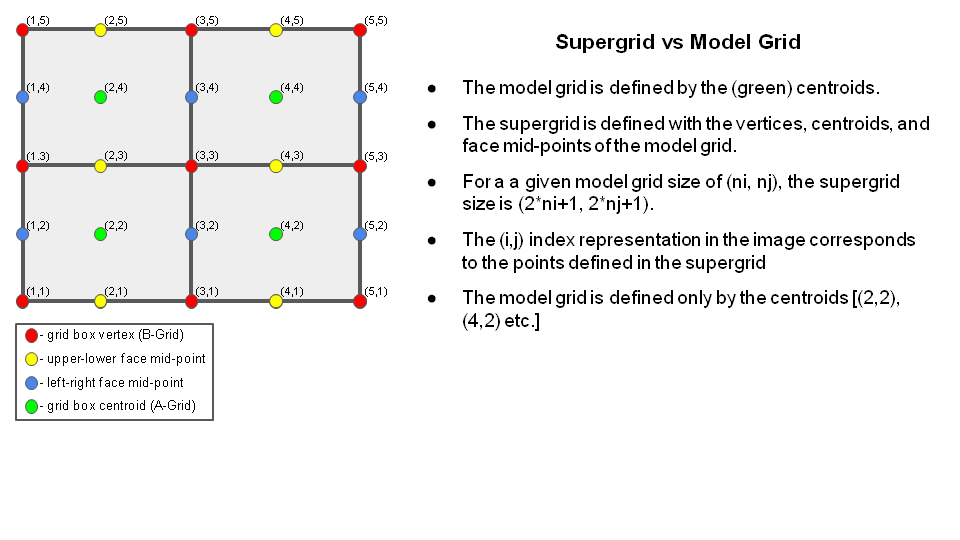
The make_hgrid program computes geo-referencing parameters for global uniform grids. (Extended Schmidt gnomonic regional grids are created by the regional_esg_grid program.) The parameters include geographic latitude and longitude, and grid cell area. See the output data section for a full list of parameters. Grids are gnomonic such that all great circles are straight lines. The parameters are computed on the staggered or “supergrid” - which has twice the resolution of the model grid. The chgres_cube initialization program maps mass fields - such as temperature - at the supergrid centroids, and u/v winds at the face mid-points. The supergrid is shown here:

3.2.2. Code Structure¶

Location of source code: ./sorc/fre-nctools.fd/tools/make_hgrid. Relevant routines:

make_hgrid.c - main driver routine

create_gnomonic_cubic_grid.c - contains routines for creating a gnomonic grid

3.2.3. Namelist Options¶

The program is controlled by these script variables:

Global uniform grid

res - x/y dimension of one tile. The “CRES” resolution. Example: a 96x96 tile would be classified as C96. It may be converted to physical resolution as follows: resol = (360 degrees / 4*CRES) * 111 km.

3.2.4. Program inputs and outputs¶

Input data:

None

Output data:

Tiled “grid” files (NetCDF) containing geo-referencing records. File naming convention: CRES_grid.tile#.nc. File records include:

x - geographic longitude (degrees)

y - geographic latitude (degrees)

dx - grid edge ‘x’ distance (m)

dy - grid edge ‘y’ distance (m)

area - grid cell area (m^2)

angle_dx - grid vertex ‘x’ angle with respect to geographic east (degrees)

angle_dy - grid vertex ‘y’ angle with respect to geographic north (degrees)

3.3. regional_esg_grid¶

3.3.1. Introduction¶

The regional_esg_grid program computes geo-referencing parameters for the Extended Schmidt Gnomonic (ESG) regional grid. The parameters include geographic latitude and longitude, and grid cell area. See the output data section for a full list of parameters. The ESG grid is designed to have nearly homogenous grid spacing. Like the make_hgrid program, the parameters are computed on the staggered or “supergrid”. For more information on the Extended Schmidt Gnomonic, see: Purser, et. al.

3.3.2. Code Structure¶

Location of source code: ./sorc/grid_tools.fd/regional_esg_grid.fd. Relevant routines:

regional_esg_grid.f90 - Main driver routine. Reads program namelist. Writes output file.

pseg.f90 - Suite of routines to perform the ESG regional grid mapping.

3.3.3. Namelist Options¶

The program is controlled by these script variables:

target_lon - center longitude of grid - degrees

target_lat - center latitude of grid - degrees

idim - dimension of grid in ‘i’ direction

jdim - dimension of grid in ‘j’ direction

delx - grid spacing in degrees in the ‘i’ direction on the supergrid. The physical grid spacing is related to delx as follows: 2*delx(circumf_earth / 360 deg).

dely - grid spacing in degrees in the ‘j’ direction on the supergrid.

halo - number of rows/cols of the lateral boundary halo

3.3.4. Program Inputs and Outputs¶

Input data:

None

Output data:

A tiled “grid” file (NetCDF) containing geo-referencing records for the supergrid. File naming convention: CRES_grid.tile7.nc. Here, CRES is the global equivalent resolution as computed by the global_equiv_resol program. Note: the forecast model assumes regional grids are tile 1. File records include:

x - geographic longitude (degrees)

y - geographic latitude (degrees)

dx - grid edge ‘x’ distance (m)

dy - grid edge ‘y’ distance (m)

area - grid cell area (m^2)

angle_dx - grid vertex ‘x’ angle with respect to geographic east (degrees)

angle_dy - grid vertex ‘y’ angle with respect to geographic north (degrees)

3.4. make_solo_mosaic¶

3.4.1. Introduction¶

This program creates the “mosaic” file, which contains information about the tiled “grid” files (such as name and tile number). For global grids, it also defines the orientation of the six tiles. All output records are listed below under “output data”. There are no runtime-selectable options for this program.

3.4.2. Code structure¶

Location of source code ./sorc/fre-nctools.fd/tools/make_solo_mosaic. Relevant routines:

make_solo_mosaic.c - main driver routine.

get_contact.c - computes the number of aligned contacts between two tiles.

3.4.3. Program inputs and outputs¶

Input data:

The tiled “grid” files (CRES_grid.tile#.nc) created by the make_hgrid or regional_esg_grid programs - (NetCDF)

Output data:

The mosaic file - CRES_mosaic.nc (NetCDF). Contains these records

Mosaic - name of mosaic (character)

Gridlocation - directory containing the “grid” files (character)

Gridfiles - names of each “grid” file (character array)

Gridtiles - list of each tile number (character array)

Contacts - list of tile contact regions - global grids only (character array)

Contact_index - list of contact regions as specified by i/j index - global grids only (character array).

3.5. global_equiv_resol¶

3.5.1. Introduction¶

This program computes the global equivalent resolution for regional grids. For example, a global grid with x/y dimensions of 96 would have a global resolution (CRES) of C96. And the approximate physical resolution would be:

Res in km = (360 degrees / 4*CRES) * 111 km = 104 km

Using the average cell size (in m^2) of the regional grid, the equivalent global resolution is computed according to:

CRES = nint( (2*pi*rad_earth)/(4*avg_cell_size) )

There are no runtime-selectable options for this program.

3.5.2. Code structure¶

Location of source code: ./sorc/grid_tools.fd/global_equiv_resol.fd. Relevant routine:

global_equiv_resol.f90 - Contains the entire program.

3.5.3. Program inputs and outputs¶

Input data:

The regional “grid” file (CRES_grid.tile#.nc) created by the regional_esg_grid program - (NetCDF). Uses the grid cell area record.

Output data:

Adds the equivalent resolution as an attribute to the “grid” file - CRES_grid.tile#.nc (NetCDF).

3.6. orog¶

3.6.1. Introduction¶

This program computes the land mask, land fraction, orography and gravity wave drag (GWD) fields on the model grid. See the output data section for a complete list of fields.

Land-sea mask and land fraction are created from a global 30-arc second University of Maryland land cover (land/non-land flag) dataset. Land fraction is determined by averaging all 30-second land cover points located within the model grid box. Points with a land fraction of 50% or more are given a land-sea mask of “land”. Orography and GWD fields are created from two datasets: 1) 30-arc-second USGS GMTED2010 orography data; 2) for Antarctica, 30-arc-second RAMP terrain data (Radarsat Antarctic Mapping Project). Fields are determined from all 30-arc second data located within the model grid box. The orography is simply the average of the 30-arc second values. It is later filtered by the filter_topo program. For details on the GWD fields, see:

Kim, Y-J and A. Arakawa, 1995: Improvement of orographic gravity wave parameterization using a mesoscale gravity wave model. J. Atmos. Sci. 52, pp 1875-1902.

Lott, F. and M. J. Miller: 1977: A new sub-grid scale orographic drag parameterization: Its formulation and testing, QJRMS, 123, pp 101-127.

Caution: At model grid resolutions of 1 km, the 30-arc-second input data will not be sufficient to properly resolve the land-sea mask, land fraction and orography fields. At model grid resolutions finer than 3 km, the remaining fields (used by the GWD) will not be well resolved. In that case, users should consider not running with GWD.

3.6.2. Code structure¶

The source code is located - ./sorc/orog_mask_tools.fd/orog.fd. Some important subroutines:

MAKEMT2 - computes land fraction, land-sea mask, orography, standard deviation of orography, and convexity.

MAKEPC2 - computes anisotropy (gamma), slope of orography (sigma) and mountain range angle (theta).

MAKEOA2 - computes maximum height (elvmax), orographic asymmetry (oa) and length scale (ol).

3.6.3. Program inputs and outputs¶

Input data:

The “grid” files (CRES_grid.tile#.nc) containing the geo-reference records for the grid - (NetCDF). Created by the make_hgrid or regional_esg_grid programs.

Global 30-arc-second University of Maryland land cover data. Used to create the land-sea mask.

landcover.umd.30s.nc (NetCDF). Located here ./fix/fix_orog.

Global 30-arc-second USGS GMTED2010 orography data.

topography.gmted2010.30s.nc (NetCDF). Located here ./fix/fix_orog.

30-arc-second RAMP Antarctic terrain data (Radarsat Antarctic Mapping Project)

topography.antarctica.ramp.30s.nc (NetCDF). Located here ./fix/fix_orog.

Output data:

Orography files - one for each tile - oro.CRES.tile#.nc (NetCDF). Contains these records:

geolon - longitude (degrees east)

geolat - latitude (degrees north)

slmsk - land-sea mask (0 - nonland; 1 - land)

land_frac - land fraction (percent)

orog_raw - orography (meters)

orog_filt - same as orog_raw

stddev - standard deviation of orography (meters)

convexity - orographic convexity (unitless)

oa[1-4] - orographic asymmetry - four directional components - W/S/SW/NW

ol[1-4] - orographic length scale - four directional components - W/S/SW/NW

theta - angle of mountain range with respect to east (degrees)

gamma - anisotropy (unitless)

sigma - slope of orography (unitless)

elvmax - maximum height above mean (meters)

3.7. orog_gsl¶

3.7.1. Introduction¶

This program computes orographics statistics fields required for the orographic drag suite developed by NOAA’s Global Systems Laboratory (GSL). The fields are a subset of the ones calculated by “orog” and are calculated in a different manner.

3.7.2. Code structure¶

Location of source code: ./sorc/orog_mask_tools.fd/orog_gsl.fd.

3.7.3. Program inputs and outputs¶

The program reads the tile number (1-6 for global, 7 for stand-alone regional) and grid resolution (e.g., 768) from standard input.

Input data:

All in NetCDF.

The tiled “grid” files (CRES_grid.tile#.nc) created by the make_hgrid or regional_esg_grid programs.

geo_em.d01.lat-lon.2.5m.HGT_M.nc - global topographic data on 2.5-minute lat-lon grid (interpolated from GMTED2010 30-second topographic data). Located here.

HGT.Beljaars_filtered.lat-lon.30s_res.nc - global topographic data on 30-second lat-lon grid (GMTED2010 data smoothed according to Beljaars et al. (QJRMS, 2004)). Located here.

Output data:

One for each tile. All in NetCDF.

CRES_oro_data_ls.tile#.nc - Large-scale file for the gravity wave drag and blocking schemes of Kim and Doyle (2005)

CRES_oro_data.ss.tile#.nc - Small-scale file for the gravity wave drag scheme of Tsiringakis et al. (2017). And the turbulent orographic from drag (TOFD) schemem of Beljaars et al. (QJRMS, 2004).

Each file contains the following records:

geolon - longitude (degrees east)

geolat - latitude (degrees north)

stddev - Standard deviation of subgrid topography

convexity - Convexity of subgrid topography

oa1 - Orographic asymmetry of subgrid topography - westerly

oa2 - Orographic asymmetry of subgrid topography - southerly

oa3 - Orographic asymmetry of subgrid topography - southwesterly

oa4 - Orographic asymmetry of subgrid topography - northwesterly

ol1 - Orographic effective length of subgrid topography - westerly

ol2 - Orographic effective length of subgrid topography - southerly

ol3 - Orographic effective length of subgrid topography - southwesterly

ol4 - Orographic effective length of subgrid topography - northwesterly

3.8. inland¶

3.8.1. Introduction¶

This program reads an orography file, determines which points are inland from water, then writes out a mask record that identifies these points.

3.8.2. Code structure¶

Location of source code: ./sorc/orog_mask_tools.fd/inland.fd.

3.8.3. Program control options¶

The program reads the following parameters from standard input:

The resolution. Ex: ‘96’ for C96.
Nonland cutoff fraction. Default is ‘0.99’.
Maximum recursive depth. Default is ‘7’.
Grid type flag - ‘g’ for global, ‘r’ for regional.

3.8.4. Program inputs and outputs¶

Input data:

orography file - The orography file from the orog program - oro.CRES.tile#.nc (NetCDF)

Output data:

orography file - The input file, but containing an additional ‘inland’ record - ‘1’ inland, ‘0’ coastal.

3.9. lakefrac¶

3.9.1. Introduction¶

This program sets freshwater lake fraction and lake depth on the model grid.

3.9.2. Code structure¶

Location of source code: ./sorc/orog_mask_tools.fd/lake.fd.

3.9.3. Program control options¶

The program reads the following parameters from standard input:

The tile number.
The resolution. Ex: ‘96’ for C96.
The path to the global lake data.
Minimum lake fraction in percent.

3.9.4. Program inputs and outputs¶

Input data:

grid file - the “grid” file from the make_hgrid or regional_esg programs - CRES_grid.tile#.nc - (NetCDF)

orography file - the orography file including the ‘inland’ flag record from the inland program - oro.CRES.tile#.nc (NetCDF)

lake status code file - One of the following files. (located in ./fix/fix_orog). See GlobalLakeStatus.txt for a description of the file format.

GlobalLakeStatus_MOSISp.dat

GlobalLakeStatus_GLDBv3release.dat

GlobalLakeStatus_VIIRS.dat

lake depth file - One of the following files. (located in ./fix/fix_orog). See GlobalLakeDepth.txt for a description of this file.

GlobalLakeDepth_GLDBv3release.dat

GlobalLakeDepth_GLOBathy.dat

Output data:

orography file - the orography file including records of lake fraction and lake depth - oro.CRES.tile#.nc (NetCDF)

3.10. filter_topo¶

3.10.1. Introduction¶

The FV3 terrain filtering algorithm has several unique properties compared to conventional topography filters. The resulting topography filtered by this algorithm has conserved globally integrated elevations. More importantly, this filter has the following island-preserving properties: 1) No Gibbs ringing at the coastlines where discontinuities occur; 2) the filtered terrain’s coastlines strictly match the source terrain’s. The detailed implementation of this terrain filtering algorithm will be described in a forthcoming publication by Dr. Shian-Jiann Lin and his group.

3.10.2. Code structure¶

Location of source code: ./sorc/grid_tools.fd/filter_topo.fd. The entire program is contained in filter_topo.F90.

3.10.3. Namelist options¶

Program execution is controlled via a namelist. The namelist variables are:

topo_file - Name of the orography file (See input data) (character)

topo_field - Name of the filtered orography record in the orography file (“orog_filt”) (character)

mask_field - Name of the land-sea mask record in the orography file (“land_frac”) (character)

grid_file - The mosaic file (See input data) (character)

zero_ocean - Flag to turn on the “island-preserving” property. Default is true (logical)

stretch_fac - Stretching factor. Equal to “1” for global uniform grids. Not applicable for ESG regional grids (floating point)

res - The “CRES” resolution (floating point)

grid_type - 0 for a gnomonic grid (integer)

regional - True for an ESG regional grid (logical)

3.10.4. Program inputs and outputs¶

Input data:

mosaic file - the mosaic file from the make_solo_mosaic program - CRES_mosaic.nc (NetCDF)

grid file - the “grid” file from the make_hgrid or regional_esg programs - CRES_grid.tile#.nc - (NetCDF)

orography file - the orography file from the orog program - oro.CRES.tile#.nc (NetCDF)

Output data:

The filtered orography is written to the “orog_filt” record of the input orography file - oro.CRES.tile#.nc (NetCDF).

3.10.5. Filtering parameters¶

n_del2 - Second-order strong filtering coefficient.

n_del2_weak - Second-order weak filtering coefficient - used to more finely smooth the topography compared to the strong filter.

cd4 - dimensionless coefficient for delta-4 diffusion.

peak_fac - overshoot factor for the mountain peak

max_slope - maximum allowable terrain slope

3.11. shave¶

3.11.1. Introduction¶

The “grid” and “orography” files for regional grids are first created with rows and columns extending beyond the halo. This is required for the topography filtering code to work correctly in the halo region. After filtering, the shave program removes these extra points from the files.

3.11.2. Code structure¶

Location of the source code: ./sorc/grid_tools.fd/shave.fd. The entire program is contained in shave_nc.F90.

3.11.3. Program control options¶

The program is controlled by these parameters read from standard input:

The i/j dimensions of the compute domain (not including halo) (integer)

The number of halo rows/columns (integer)

The file name with the extra points (character string)

The name of the output file with the extra points removed (character string)

3.11.4. Program inputs and outputs¶

Input data:

Model “grid” files (CRES_grid.tile#.nc) created by the make_hgrid or regional_esg_grid programs - (NetCDF)

Model orography files (oro.CRES.tile#.nc) after topography filtering - (NetCDF)

Output data:

With and without the halo.

Model “grid” files - CRES.grid.tile#.halo#.nc (NetCDF)

Model orography files - CRES.oro_data.tile#.halo#.nc (NetCDF)

3.12. sfc_climo_gen¶

3.12.1. Introduction¶

The sfc_climo_gen (surface climatological field generation) program creates surface climatological fields such as soil type, vegetation type and albedo. Some fields may be time-varying: for example, snow-free albedo is monthly. But they are static - i.e., they only need to be generated when the grid is created. The program uses the ESMF library to horizontally interpolate the source data to the model grid. For regional grids, the program will output files with and without the halo region when the “halo” namelist variable is set.

3.12.2. Code structure¶

Location of the source code: ./sorc/sfc_climo_gen.fd. Brief description of each module:

driver.F90 - The main driver routine.

interp.F90 - The interpolation driver routine. Reads the input source data and interpolates it to the model grid.

interp_frac_cats.F90 - Same as interp.F90, but for computing the fraction of each soil and vegetation type category. (When namelist variable ‘vegsoilt_frac’ is true).

model_grid.F90 - Defines the ESMF grid object for the model grid.

output.f90 - Writes the output surface data to a NetCDF file. For regional grids, will output separate files with and without the halo.

output_frac_cats.f90 - Same as output.f90, but for writing fractional soil and vegetation type. (When namelist variable ‘vegsoilt_frac’ is true).

program_setup.f90 - Reads the namelist and sets up program execution.

search.f90 - Replace undefined values on the model grid with a valid value at a nearby neighbor. Undefined values are typically associated with isolated islands where there is no source data.

search_frac_cats.f90 - Same as search.f90, but for the fractional soil and vegetation type option. (When namelist variable ‘vegsoilt_frac’ is true).

source_grid.F90 - Reads the grid specifications and land/sea mask for the source data. Sets up the ESMF grid object for the source grid.

utils.f90 - Contains error handling utility routines.

3.12.3. Namelist options¶

Program execution is controlled via a namelist. The namelist variables are:

input_facsf_file - path/name of input fractional strong/weak zenith angle albedo data

input_substrate_file - path/name of input soil substrate temperature data

input_maximum_snow_albedo_file - path/name of input maximum snow albedo data

input_snowfree_albedo_file - path/name of input snow-free albedo data

input_slope_type_file - path/name of input global slope type data

input_soil_type_file - path/name of input soil type data

input_soil_color_file - path/name of input soil color data

input_vegetation_type_file - path/name of vegetation type data

input_vegetation_greenness_file - path/name of monthly vegetation greenness data

mosaic_file_mdl - path/name of the model mosaic file

orog_dir_mdl - directory containing the model orography files

orog_files_mdl - list of model orography files. For global uniform grids, all six files are listed.

halo - number of rows/cols of the lateral boundary halo (regional grids only). When selected, the program will output files with and without the halo region.

maximum_snow_albedo_method - interpolation method for this field. Bilinear or conservative. Default is bilinear.

snowfree_albedo_method - interpolation method for this field. Bilinear or conservative. Default is bilinear.

vegetation_greenness_method - interpolation method for this field. Bilinear or conservative. Default is bilinear.

vegsoilt_frac - When ‘true’, outputs the dominate soil and vegetation type, and the fraction of each category. When ‘false’, only outputs the dominate categories. Default is ‘false’.

3.12.4. Program inputs and outputs¶

Input data:

The surface climatological data is located here ./fix/fix_sfc_climo. All NetCDF.

Global 1-degree fractional coverage strong/weak zenith angle albedo - facsf.1.0.nc

Global 0.05-degree maximum snow albedo - maximum_snow_albedo.0.05.nc

Global 0.5-degree soil substrate temperature - substrate_temperature.gfs.0.5.nc

Global 0.05-degree four component monthly snow-free albedo - snowfree_albedo.4comp.0.05.nc

Global 1.0-degree categorical slope type - slope_type.1.0.nc

Global 0.05-degree CLM soil color (Lawrence and Chase, 2007 JGR) - soil_color.clm.0.05.nc

Categorical STATSGO soil type

Global 0.05-degree - soil_type.statsgo.0.05.nc

Global 0.03-degree - soil_type.statsgo.0.03.nc

CONUS 30 sec - soil_type.statsgo.conus.30s.nc

N Hemis 30 sec - soil_type.statsgo.nh.30s.nc

Global 30 sec - soil_type.statsgo.30s.nc

Categorical BNU soil type

Global 30-second - soil_type.bnu.v3.30s.nc

Categorical IGBP vegetation type

MODIS-based global 0.05-degree - vegetation_type.modis.igbp.0.05.nc

MODIS-based global 0.03-degree - vegetation_type.modis.igbp.0.03.nc

MODIS-based CONUS 30 sec - vegetation_type.modis.igbp.conus.30s.nc

MODIS-based N Hemis 30 sec - vegetation_type.modis.igbp.nh.30s.nc

MODIS-based global 30 sec - vegetation_type.modis.igbp.30s.nc

NESDIS VIIRS-based global 30-second - vegetation_type.viirs.v3.igbp.30s.nc

Global 0.144-degree monthly vegetation greenness in percent - vegetation_greenness.0.144.nc

The files that define the model grid. All NetCDF.

Model mosaic file - CRES_mosaic.nc

Model orography files including halo - CRES_oro_data.tile#.halo#.nc

Model grid files including halo - CRES_grid.tile#.halo#.nc

Output files:

All files with and without halo (all NetCDF).

Fractional coverage strong/weak zenith angle albedo - CRES_facsf.tile#.halo#.nc

Maximum snow albedo - CRES_maximum_snow_albedo.tile#.halo#nc

Soil substrate temperature - CRES_substrate_temperature.tile#.halo#.nc

Snow free albedo - CRES_snowfree_albedo.tile#.halo#.nc

Slope type - CRES_slope_type.tile#.halo#.nc

Soil type - CRES_soil_type.tile#.halo#.nc

Soil color - CRES_soil_color.tile#.halo#.nc

Vegetation type - CRES_vegetation_type.tile#.halo#.nc

Vegetation greenness - CRES_vegetation_greenness.tile#.halo#.nc

3.13. vcoord_gen¶

3.13.1. Introduction¶

This program generates hybrid coordinate parameters from fields such as surface pressure, model top and the number of vertical levels. Outputs the ‘ak’ and ‘bk’ parameters used by the forecast model and chgres_cube to define the hybrid levels as follows:

pressure = ak + (surface_pressure * bk)

3.13.2. Code structure¶

Location of the source code: ./sorc/vcoord_gen.fd.

3.13.3. Program inputs¶

The following user-defined parameters are read in from standard input.

levs - Integer number of levels

lupp - Integer number of levels below pupp

pbot - Real nominal surface pressure (Pa)

psig - Real nominal pressure where coordinate changes from pure sigma (Pa)

ppre - Real nominal pressure where coordinate changes from pure pressure (Pa)

pupp - Real nominal pressure where coordinate changes to upper atmospheric profile (Pa)

ptop - Real pressure at top (Pa)

dpbot - Real coordinate thickness at bottom (Pa)

dpsig - Real thickness of zone within which coordinate changes to pure sigma (Pa)

dppre - Real thickness of zone within which coordinate changes to pure pressure (Pa)

dpupp - Real coordinate thickness at pupp (Pa)

dptop - Real coordinate thickness at top (Pa)

3.13.4. Program outputs¶

A text file is output containing the ‘ak’ and ‘bk’ values. To use it in chgres_cube, set namelist variable “vcoord_target_grid” to the path/name of this file.

3.13.5. Run script¶

To run, use script ./util/vcoord_gen/run.sh

3.14. weight_gen¶

3.14.1. Introduction¶

Creates ESMF ‘scrip’ files for gaussian grids.

3.14.2. Code structure¶

Location of the source code: ./sorc/weight_gen.fd.

3.14.3. Program inputs¶

The global FV3 grid resolution from standard output. Valid choices are:

C48

C96

C128

C192

C384

C768

C1152

C3072

3.14.4. Program outputs¶

Two gaussian grid ‘scrip’ files in NetCDF format. One includes two extra rows for the poles.

C48 => 192x94 and 192x96 gaussian files

C96 => 384x192 and 384x194 gaussian files

C128 => 512x256 and 512x258 gaussian files

C192 => 768x384 and 768x386 gaussian files

C384 => 1536x768 and 1536x770 gaussian files

C768 => 3072x1536 and 3072x1538 gaussian files

C1152 => 4608x2304 and 4608x2406 gaussian files

C3072 => 12288x6144 and 12288x6146 gaussian files

Files contain center and corner point latitude and longitudes.

3.14.5. Run script¶

To run, use the machine-dependent script under ./util/weight_gen

4. UFS_UTILS utilities¶

4.1. gdas_init¶

4.1.1. Introduction¶

The gdas_init utility is used to create coldstart initial conditions for global cycled and forecast-only experiments using the chgres_cube program. It has two components: one that pulls the input data required by chgres_cube from HPSS, and one that runs chgres_cube. The utility is only supported on machines with access to HPSS:

Hera

Jet

WCOSS2

S4 (Only the chgres_cube step is supported, not the data pull step.)

4.1.2. Location¶

Find it here: ./util/gdas_init

4.1.3. Build UFS_UTILS and set ‘fixed’ directories¶

Invoke the build script from the root directory:

./build_all.sh

Set the ‘fixed’ directories using the script in the ‘./fix’ subdirectory (where $MACHINE is ‘hera’, ‘jet’, ‘wcoss2’, or ‘s4’):

./link_fixdirs.sh emc $MACHINE

4.1.4. Configure for your experiment¶

Edit the variables in the ‘config’ file for your experiment:

EXTRACT_DIR - Directory where data extracted from HPSS is stored.

EXTRACT_DATA - Set to ‘yes’ to extract data from HPSS. If data has been extracted and is located in EXTRACT_DIR, set to ‘no’. On ‘s4’ this step can’t be run. Instead, the data must be pulled from another machine.

RUN_CHGRES - To run chgres, set to ‘yes’. To extract data only, set to ‘no’.

yy/mm/dd/hh - The year/month/day/hour of your desired experiment. Use a four digit year and two digits for month/day/hour. NOTE: The standard build of chgres_cube does NOT support experiments prior to June 12, 2019. To coldstart an experiment prior to these dates, contact a repository manager for assistance.

LEVS - Number of hybrid levels plus 1. To run with 127 levels, set LEVS to 128.

CRES_HIRES - Resolution of the hires component of your experiment. Example: C768.

CRES_ENKF - Resolution of the enkf component of the experiments.

UFS_DIR - Location of your cloned UFS_UTILS repository.

OUTDIR - Directory where the coldstart data output from chgres is stored.

CDUMP - When ‘gdas’, will process gdas and enkf members. When ‘gfs’, will process gfs member for running free forecast only.

use_v16retro - When ‘yes’, use v16 retrospective parallel data. The retrospective parallel tarballs can be missing or incomplete. So this option may not always work. Contact a UFS_UTILS repository manager if you encounter problems.

Note: This utility selects the ocean resolution in the set_fixed_files.sh script using a default based on the user-selected CRES value. For example, for a cycled experiment with a CRES_HIRES/CRES_ENKF of C384/C192, the ocean resolution defaults to 0.25/0.50-degree. To choose another ocean resolution, the user will need to manually modify the set_fixed_files.sh script.

4.1.5. Kick off the utility¶

Submit the driver script (where $MACHINE is ‘hera’, ‘jet’, ‘wcoss2’, or ‘s4’)

./driver.$MACHINE.sh

The standard output will be placed in log files in the current directory.

The converted output will be found in $OUTDIR, including the needed abias and radstat initial condition files (if CDUMP=gdas). The files will be in the needed directory structure for the global-workflow system, therefore a user can move the contents of their $OUTDIR directly into their $ROTDIR.